Visualising RDMs with the 92 images dataset

This notebook demonstrates how rsatoolbox.vis.show_rdm can be used to visualise RDMs. By setting the RDM’s pattern_descriptors to rsatoolbox.vis.Icon instances it is possible to automatically generate stacked image labels and other custom visualisations.

# imports
import matplotlib.pyplot as plt
import matplotlib
from rsatoolbox import vis
from rsatoolbox import rdm
import numpy as np
import os
import inspect
import scipy.io
from collections import defaultdict

Loading data and building RDMs instance with Icon pattern_descriptors

Before we begin, we need to load up the fMRI data from the 92 images dataset (Kriegeskorte et al., 2008).

# supporting functions and constants
DEMO_DIR = os.getcwd()
NEURON_DIR = os.path.join(DEMO_DIR, "92imageData")


def neuron_2008_icons(**kwarg):
    """ Load Krigeskorte et al. (2008, Neuron) images as Icon instances."""
    mat_path = os.path.join(NEURON_DIR, "Kriegeskorte_Neuron2008_supplementalData.mat")
    mat = scipy.io.loadmat(mat_path)
    colors = plt.get_cmap('Accent', lut=16).colors
    markers = list(matplotlib.markers.MarkerStyle('').markers.keys())
    icons = defaultdict(list)
    for this_struct in mat["stimuli_92objs"][0]:
        # we're going to treat the 4 binary indicators (human, face, animal, natural) as a
        # base2 binary string, and index into this array of colors accordingly.
        index = int("".join(
                     [
                         str(this_struct[this_key][0,0]) for this_key in (
                     'human', 'face', 'animal', 'natural')
                     ]
                 ),
                                  base=2)
        this_color = colors[index]
        icons['image'].append(vis.Icon(image=this_struct['image'],
                                       color=this_color,
                                       circ_cut='cut',
                                       border_type='conv',
                                       border_width=5,
                                       **kwarg))
        icons['string'].append(vis.Icon(string=this_struct['category'][0],
                                        color=this_color,
                                        font_color=this_color,
                                        **kwarg))
        icons['marker'].append(vis.Icon(marker=markers[index],
                                       color=this_color,
                                       **kwarg))
    return icons


def neuron_2008_rdms_fmri(**kwarg):
    """ Load Kriegeskorte et al. (2008, Neuron) fMRI RDMs as RDMs instance.
    All key-word arguments are passed to neuron_2008_images."""
    mat_path = os.path.join(NEURON_DIR, "92_brainRDMs.mat")
    mat = scipy.io.loadmat(mat_path)
    icons = neuron_2008_icons(**kwarg)
    # insert leading dim to conform with rsatoolbox nrdm x ncon x ncon convention
    return rdm.concat(
        [
            rdm.RDMs(
                dissimilarities=this_rdm["RDM"][None, :, :],
                dissimilarity_measure="1-rho",
                rdm_descriptors=dict(
                    zip(["ROI", "subject", "session"], this_rdm["name"][0].split(" | ")),
                    name=this_rdm["name"][0]
                ),
                pattern_descriptors=icons
            )
            for this_rdm in mat["RDMs"].flatten()
        ]
    )

# as an example, load the Kriegeskorte et al., 2008 fMRI RDMs
rdms = neuron_2008_rdms_fmri()

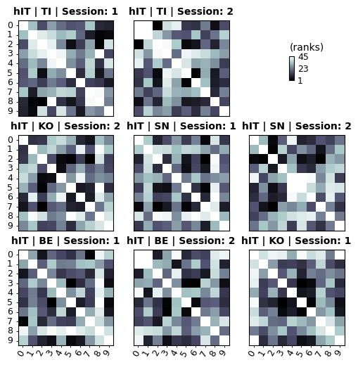
Plotting RDMs with text labels

# to keep it simple, let's start with plotting the first 10 conditions
rdms_small = rdms.subset_pattern('index', np.arange(10))
rdms_small = rdm.rank_transform(rdms_small)

vis.show_rdm(rdms_small, rdm_descriptor='name', show_colorbar='figure', pattern_descriptor='index')
plt.show()

Plotting with image labels

It might help to put some image labels on…

vis.show_rdm(rdms_small,
             rdm_descriptor='name',
             show_colorbar='figure',
             pattern_descriptor='image')
plt.show()

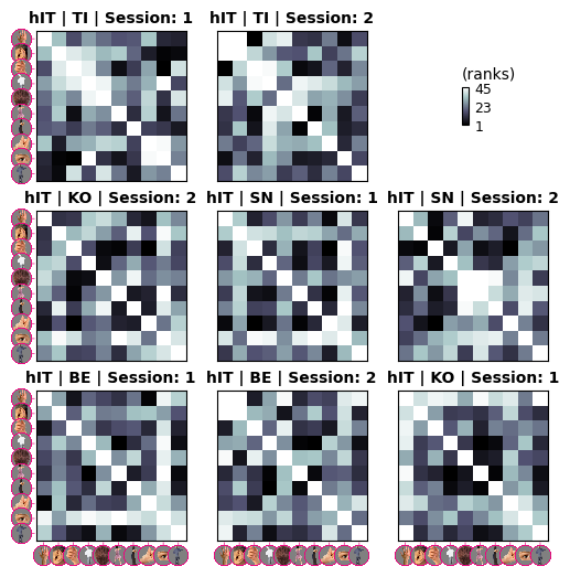
Notice how the image labels are scaled to avoid overlap. However, they are rather small. Grouping them might help us get away with larger images. We will also tweak icon_spacing to 10% overlap between the images.

vis.show_rdm(rdms_small,
             rdm_descriptor='name',
             show_colorbar='figure',
             pattern_descriptor='image',
            num_pattern_groups=5,
            icon_spacing=.9)
plt.show()

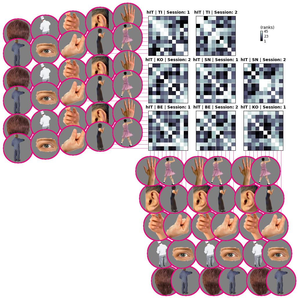
Now the images are very clear (maybe too big in fact, unless you are preparing a figure for a slideshow). Notice how show_rdm adds white gridlines to mark the label groups. If you like, you can control this behavior with the gridlines argument.

For now though, let’s scale up to the full insanity of 92 images…

# probably sane not to plot too many of these
fig, ax, ret_val = vis.show_rdm(rdms[0],
             rdm_descriptor='name',
             pattern_descriptor='image',
             num_pattern_groups=6,
             icon_spacing=.9,
             show_colorbar='panel',
             vmin=0.,
             n_column=1,
             figsize=(10,10)
            )
plt.show()

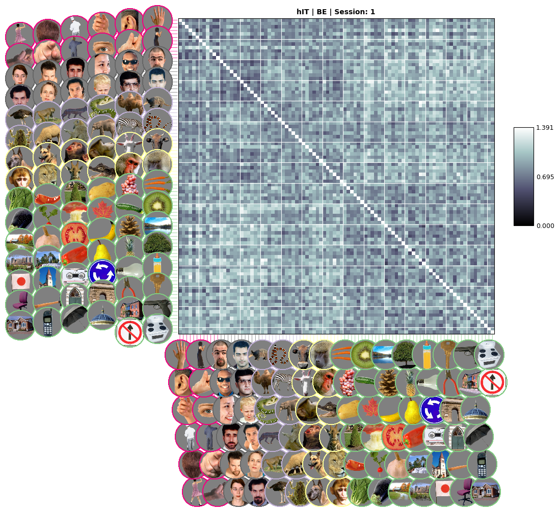
Not too bad, considering how many images we are plotting. With this full view you can also see two other features that help guide the eye in large RDM visualisations: * A carefully selected num_pattern_groups parameter really helps with picking out interesting conditions (notice how the faces are in grids 3-4 and 7-8 above). * The color parameter that was used when instancing the Icons controls the color of the supporting lines and the circular outlines. This can also be used to convey category membership.

Optimising image label display and saving figure

In general, you can achieve larger, clearer image labels by * plotting fewer RDMs in the same figure * increasing num_pattern_groups * decreasing icon_spacing * adjusting figsize * increasing dpi when saving, see below

# to save the figure, remember to set bbox_inches='tight'.
# (Otherwise the image labels may get cropped out)
fig.savefig('temp_rdm.png', bbox_inches='tight', dpi=300)

The saved RDM image is plotted below. It may look quite a bit crisper than the inline view we generated previously.

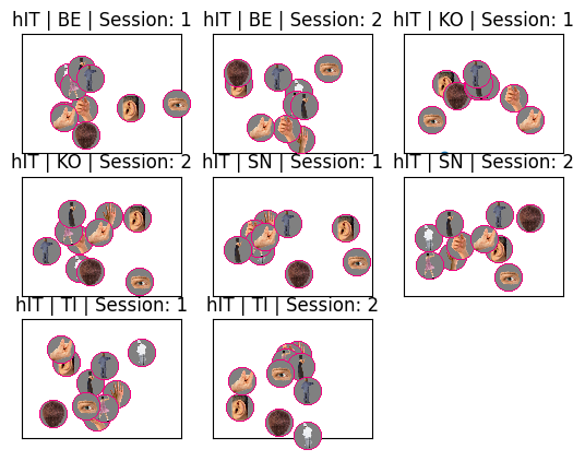
Plot MDS

Here we make a scatterplot of the RDM reduced to two dimensions using MultiDimensional Scaling

vis.show_MDS(
    rdms_small,
    rdm_descriptor='name',
    pattern_descriptor='image'
)