Temporal RSA¶

This demo notebook demonstrates how to work with temporal data in the RSA toolbox

So far, it demonstrates how to

import temporal dataset into the rsatoolbox.data.TemporalDataset class and
how to create RDM movies using the rsatoolbox.rdm.calc_rdm_movie function

The notebook will

[1]:

import numpy as np
import matplotlib.pyplot as plt
import rsatoolbox
import pickle

from rsatoolbox.rdm import calc_rdm_movie

Load temporal data¶

I here used sample data from mne-python

https://mne.tools/dev/overview/datasets_index.html#sample

Data is comprised of the preprocessed MEG data in “sample_audvis_raw.fif”.

Preprocessing includes: - downsampling to 60Hz - band-pass filtering between 1 Hz and 20 Hz - rejecting bad trials using an amplitude threshold - baseline correction (basline -200 to 0 ms)

See demos/TemporalSampleData/preproc_mn_sample_data.py

The preprocessed data is stored in TemporalSampleData/meg_sample_data.pkl

[2]:

dat = pickle.load( open( "TemporalSampleData/meg_sample_data.pkl", "rb" ) )
measurements = dat['data']
cond_names = [x for x in dat['cond_names'].keys()]
cond_idx = dat['cond_idx']
channel_names = dat['channel_names']
times = dat['times']

[3]:

print('there are %d observations (trials), %d channels, and %d time-points\n' %
      (measurements.shape))

print('conditions:')
print(cond_names)

there are 227 observations (trials), 203 channels, and 58 time-points

conditions:
['Auditory/Left', 'Auditory/Right', 'Visual/Left', 'Visual/Right']

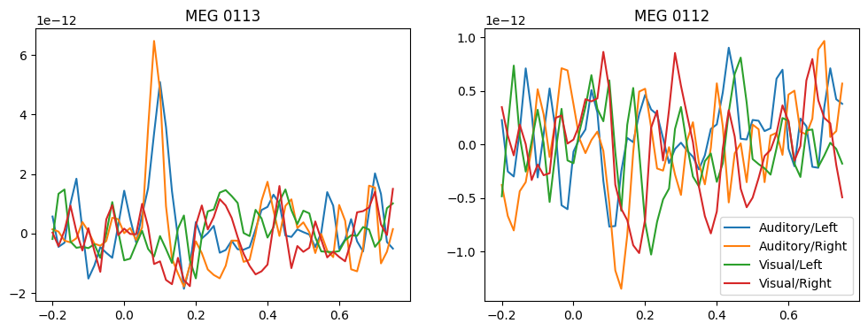
Plot condition averages for two channels:

[4]:

fig, ax = plt.subplots(1, 2, figsize=(12,4))
ax = ax.flatten()
for jj,chan in enumerate(channel_names[:2]):
    for ii, cond_ii in enumerate(np.unique(cond_idx)):
        mn = measurements[cond_ii == cond_idx,jj,:].mean(0).squeeze()
        ax[jj].plot(times, mn, label = cond_names[ii])
        ax[jj].set_title(chan)
ax[jj].legend()
plt.show()

The `rsatoolbox.data.TemporalDataset` class¶

measurements is an np.array of shape n_obs x n_channels x n_times

time_descriptor should contain the time-point vector for the measurements of length n_times. it is recommended to call this descriptor ‘time’

[5]:

tim_des = {'time': times}

the other descriptors are identical as in the rsatoolbox.data.Dataset class

[6]:

des = {'session': 0, 'subj': 0}
obs_des = {'conds': cond_idx}
chn_des = {'channels': channel_names}

[7]:

data = rsatoolbox.data.TemporalDataset(measurements,
                              descriptors = des,
                              obs_descriptors = obs_des,
                              channel_descriptors = chn_des,
                              time_descriptors = tim_des)
data.sort_by('conds')

convenience methods¶

rsatoolbox.data.TemporalDataset comes with the same convenience methods as rsatoolbox.data.Dataset.

In addition, the following functions are provided:

rsatoolbox.data.TemporalDataset.split_time(by)
rsatoolbox.data.TemporalDataset.subset_time(by, t_from, t_to)
rsatoolbox.data.TemporalDataset.bin_time(by, bins)
rsatoolbox.data.TemporalDataset.time_as_observations(by)

`rsatoolbox.data.TemporalDataset.split_time(by)`¶

splits the rsatoolbox.data.TemporalDataset object into a list of n_times rsatoolbox.data.TemporalDatset objects, splitting the measurements along the time_descriptor by

[8]:

print('shape of original measurements')
print(data.measurements.shape)

data_split_time = data.split_time('time')

print('\nafter splitting')
print(len(data_split_time))
print(data_split_time[0].measurements.shape)

shape of original measurements
(227, 203, 58)

after splitting
58
(227, 203, 1)

`rsatoolbox.data.TemporalDataset.subset_time(by, t_from, t_to)`¶

returns a new rsatoolbox.data.TemporalDataset with only the data between where time_descriptors[by] is between t_from and t_to

[9]:

print('shape of original measurements')
print(data.measurements.shape)

data_subset_time = data.subset_time('time', t_from = -.1, t_to = .5)

print('\nafter subsetting')
print(data_subset_time.measurements.shape)
print(data_subset_time.time_descriptors['time'][0])

shape of original measurements
(227, 203, 58)

after subsetting
(227, 203, 37)
-0.09989760657919393

`rsatoolbox.data.TemporalDataset.bin_time(by, bins)`¶

returns a new rsatoolbox.data.TemporalDataset object with binned temporal data. data within bins is averaged.

bins is a list or array, where the first dimension contains the bins, and the second dimension the old time-bins that should go into this bin.

[10]:

bins = np.reshape(tim_des['time'], [-1, 2])
print(len(bins))
print(bins[0])

29
[-0.19979521 -0.18314561]

[11]:

print('shape of original measurements')
print(data.measurements.shape)

data_binned = data.bin_time('time', bins=bins)

print('\nafter binning')
print(data_binned.measurements.shape)
print(data_binned.time_descriptors['time'][0])

shape of original measurements
(227, 203, 58)

after binning
(227, 203, 29)
-0.1914704126101217

`rsatoolbox.data.TemporalDataset.time_as_observations(by)`¶

returns a rsatoolbox.data.Dataset object where the time dimension is absorbed into the observation dimension

[12]:

print('shape of original measurements')
print(data.measurements.shape)

data_dataset = data.time_as_observations('time')

print('\nafter binning')
print(data_dataset.measurements.shape)
print(data_dataset.obs_descriptors['time'][0])

shape of original measurements
(227, 203, 58)

after binning
(13166, 203)
-0.19979521315838786

create RDM movie¶

the function calc_rdm_movie takes rsatoolbox.data.TemporalDataset as an input and outputs an RDMs rsatoolbox.rdm.RDMs object. It works like calc_rdm.

[13]:

rdms_data = calc_rdm_movie(data, method = 'euclidean',
                           descriptor = 'conds')
print(rdms_data)

rsatoolbox.rdm.RDMs
58 RDM(s) over 4 conditions

dissimilarity_measure =
squared euclidean

dissimilarities[0] =
[[0.00000000e+00 4.48201826e-25 6.17620803e-25 4.68172301e-25]
 [4.48201826e-25 0.00000000e+00 7.16414642e-25 4.27861898e-25]
 [6.17620803e-25 7.16414642e-25 0.00000000e+00 7.61554453e-25]
 [4.68172301e-25 4.27861898e-25 7.61554453e-25 0.00000000e+00]]

descriptors:

rdm_descriptors:
session = [0, 0, 0, 0, 0, 0, 0, 0, 0, 0, 0, 0, 0, 0, 0, 0, 0, 0, 0, 0, 0, 0, 0, 0, 0, 0, 0, 0, 0, 0, 0, 0, 0, 0, 0, 0, 0, 0, 0, 0, 0, 0, 0, 0, 0, 0, 0, 0, 0, 0, 0, 0, 0, 0, 0, 0, 0, 0]
subj = [0, 0, 0, 0, 0, 0, 0, 0, 0, 0, 0, 0, 0, 0, 0, 0, 0, 0, 0, 0, 0, 0, 0, 0, 0, 0, 0, 0, 0, 0, 0, 0, 0, 0, 0, 0, 0, 0, 0, 0, 0, 0, 0, 0, 0, 0, 0, 0, 0, 0, 0, 0, 0, 0, 0, 0, 0, 0]
index = [0, 1, 2, 3, 4, 5, 6, 7, 8, 9, 10, 11, 12, 13, 14, 15, 16, 17, 18, 19, 20, 21, 22, 23, 24, 25, 26, 27, 28, 29, 30, 31, 32, 33, 34, 35, 36, 37, 38, 39, 40, 41, 42, 43, 44, 45, 46, 47, 48, 49, 50, 51, 52, 53, 54, 55, 56, 57]
time = [-0.19979521 -0.18314561 -0.16649601 -0.14984641 -0.13319681 -0.11654721
 -0.09989761 -0.08324801 -0.0665984  -0.0499488  -0.0332992  -0.0166496
  0.          0.0166496   0.0332992   0.0499488   0.0665984   0.08324801
  0.09989761  0.11654721  0.13319681  0.14984641  0.16649601  0.18314561
  0.19979521  0.21644481  0.23309442  0.24974402  0.26639362  0.28304322
  0.29969282  0.31634242  0.33299202  0.34964162  0.36629122  0.38294083
  0.39959043  0.41624003  0.43288963  0.44953923  0.46618883  0.48283843
  0.49948803  0.51613763  0.53278724  0.54943684  0.56608644  0.58273604
  0.59938564  0.61603524  0.63268484  0.64933444  0.66598404  0.68263364
  0.69928325  0.71593285  0.73258245  0.74923205]

pattern_descriptors:
index = [0, 1, 2, 3]
conds = [1.0, 2.0, 3.0, 4.0]

Binning can be applied before computing the RDMs by simpling specifying the bins argument

[14]:

rdms_data_binned = calc_rdm_movie(data, method = 'euclidean',
                           descriptor = 'conds',
                           bins=bins)
print(rdms_data_binned)

rsatoolbox.rdm.RDMs
29 RDM(s) over 4 conditions

dissimilarity_measure =
squared euclidean

dissimilarities[0] =
[[0.00000000e+00 3.46836229e-25 4.81401601e-25 3.27640005e-25]
 [3.46836229e-25 0.00000000e+00 4.35938622e-25 3.20443252e-25]
 [4.81401601e-25 4.35938622e-25 0.00000000e+00 5.22469051e-25]
 [3.27640005e-25 3.20443252e-25 5.22469051e-25 0.00000000e+00]]

descriptors:

rdm_descriptors:
session = [0, 0, 0, 0, 0, 0, 0, 0, 0, 0, 0, 0, 0, 0, 0, 0, 0, 0, 0, 0, 0, 0, 0, 0, 0, 0, 0, 0, 0]
subj = [0, 0, 0, 0, 0, 0, 0, 0, 0, 0, 0, 0, 0, 0, 0, 0, 0, 0, 0, 0, 0, 0, 0, 0, 0, 0, 0, 0, 0]
index = [0, 1, 2, 3, 4, 5, 6, 7, 8, 9, 10, 11, 12, 13, 14, 15, 16, 17, 18, 19, 20, 21, 22, 23, 24, 25, 26, 27, 28]
time = [-0.19147041 -0.15817121 -0.12487201 -0.09157281 -0.0582736  -0.0249744
  0.0083248   0.041624    0.0749232   0.10822241  0.14152161  0.17482081
  0.20812001  0.24141922  0.27471842  0.30801762  0.34131682  0.37461602
  0.40791523  0.44121443  0.47451363  0.50781283  0.54111204  0.57441124
  0.60771044  0.64100964  0.67430884  0.70760805  0.74090725]

pattern_descriptors:
index = [0, 1, 2, 3]
conds = [1.0, 2.0, 3.0, 4.0]

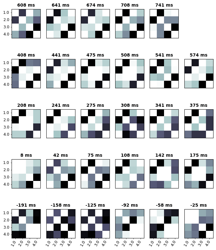
from here on¶

The following are examples for data analysis and plotting with temporal data. So far it uses the functions for non-temporal data of the toolbox. This section should be expanded once new temporal RSA functions are added to the toolbox.

I here use plotting from the standard plotting function.

[15]:

plt.figure(figsize=(10,15))

# add formated time as rdm_descriptor
rdms_data_binned.rdm_descriptors['time_formatted'] = ['%0.0f ms' % (np.round(x*1000,2)) for x in rdms_data_binned.rdm_descriptors['time']]

rsatoolbox.vis.show_rdm(rdms_data_binned,
                   pattern_descriptor='conds',
                   rdm_descriptor='time_formatted')

[15]:

(<Figure size 830x1000 with 30 Axes>,
 array([[<AxesSubplot: title={'center': '-191 ms'}>,
         <AxesSubplot: title={'center': '-158 ms'}>,
         <AxesSubplot: title={'center': '-125 ms'}>,
         <AxesSubplot: title={'center': '-92 ms'}>,
         <AxesSubplot: title={'center': '-58 ms'}>,
         <AxesSubplot: title={'center': '-25 ms'}>],
        [<AxesSubplot: title={'center': '8 ms'}>,
         <AxesSubplot: title={'center': '42 ms'}>,
         <AxesSubplot: title={'center': '75 ms'}>,
         <AxesSubplot: title={'center': '108 ms'}>,
         <AxesSubplot: title={'center': '142 ms'}>,
         <AxesSubplot: title={'center': '175 ms'}>],
        [<AxesSubplot: title={'center': '208 ms'}>,
         <AxesSubplot: title={'center': '241 ms'}>,
         <AxesSubplot: title={'center': '275 ms'}>,
         <AxesSubplot: title={'center': '308 ms'}>,
         <AxesSubplot: title={'center': '341 ms'}>,
         <AxesSubplot: title={'center': '375 ms'}>],
        [<AxesSubplot: title={'center': '408 ms'}>,
         <AxesSubplot: title={'center': '441 ms'}>,
         <AxesSubplot: title={'center': '475 ms'}>,
         <AxesSubplot: title={'center': '508 ms'}>,
         <AxesSubplot: title={'center': '541 ms'}>,
         <AxesSubplot: title={'center': '574 ms'}>],
        [<AxesSubplot: title={'center': '608 ms'}>,
         <AxesSubplot: title={'center': '641 ms'}>,
         <AxesSubplot: title={'center': '674 ms'}>,
         <AxesSubplot: title={'center': '708 ms'}>,
         <AxesSubplot: title={'center': '741 ms'}>, <AxesSubplot: >]],
       dtype=object),
 defaultdict(dict,
             {<AxesSubplot: title={'center': '-191 ms'}>: {'image': <matplotlib.image.AxesImage at 0x2c5153280>,
               'y_labels': [Text(0, 0, '1.0'),
                Text(0, 1, '2.0'),
                Text(0, 2, '3.0'),
                Text(0, 3, '4.0')],
               'x_labels': [Text(0, 0, '1.0'),
                Text(1, 0, '2.0'),
                Text(2, 0, '3.0'),
                Text(3, 0, '4.0')]},
              <AxesSubplot: title={'center': '-158 ms'}>: {'image': <matplotlib.image.AxesImage at 0x297856470>,
               'x_labels': [Text(0, 0, '1.0'),
                Text(1, 0, '2.0'),
                Text(2, 0, '3.0'),
                Text(3, 0, '4.0')]},
              <AxesSubplot: title={'center': '-125 ms'}>: {'image': <matplotlib.image.AxesImage at 0x297856950>,
               'x_labels': [Text(0, 0, '1.0'),
                Text(1, 0, '2.0'),
                Text(2, 0, '3.0'),
                Text(3, 0, '4.0')]},
              <AxesSubplot: title={'center': '-92 ms'}>: {'image': <matplotlib.image.AxesImage at 0x297f80850>,
               'x_labels': [Text(0, 0, '1.0'),
                Text(1, 0, '2.0'),
                Text(2, 0, '3.0'),
                Text(3, 0, '4.0')]},
              <AxesSubplot: title={'center': '-58 ms'}>: {'image': <matplotlib.image.AxesImage at 0x297f82a70>,
               'x_labels': [Text(0, 0, '1.0'),
                Text(1, 0, '2.0'),
                Text(2, 0, '3.0'),
                Text(3, 0, '4.0')]},
              <AxesSubplot: title={'center': '-25 ms'}>: {'image': <matplotlib.image.AxesImage at 0x297fc35b0>,
               'x_labels': [Text(0, 0, '1.0'),
                Text(1, 0, '2.0'),
                Text(2, 0, '3.0'),
                Text(3, 0, '4.0')]},
              <AxesSubplot: title={'center': '8 ms'}>: {'image': <matplotlib.image.AxesImage at 0x2c511ba90>,
               'y_labels': [Text(0, 0, '1.0'),
                Text(0, 1, '2.0'),
                Text(0, 2, '3.0'),
                Text(0, 3, '4.0')]},
              <AxesSubplot: title={'center': '42 ms'}>: {'image': <matplotlib.image.AxesImage at 0x297f50280>},
              <AxesSubplot: title={'center': '75 ms'}>: {'image': <matplotlib.image.AxesImage at 0x297e11780>},
              <AxesSubplot: title={'center': '108 ms'}>: {'image': <matplotlib.image.AxesImage at 0x297e46020>},
              <AxesSubplot: title={'center': '142 ms'}>: {'image': <matplotlib.image.AxesImage at 0x297e7a680>},
              <AxesSubplot: title={'center': '175 ms'}>: {'image': <matplotlib.image.AxesImage at 0x297eaef20>},
              <AxesSubplot: title={'center': '208 ms'}>: {'image': <matplotlib.image.AxesImage at 0x297ee7730>,
               'y_labels': [Text(0, 0, '1.0'),
                Text(0, 1, '2.0'),
                Text(0, 2, '3.0'),
                Text(0, 3, '4.0')]},
              <AxesSubplot: title={'center': '241 ms'}>: {'image': <matplotlib.image.AxesImage at 0x297dd9030>},
              <AxesSubplot: title={'center': '275 ms'}>: {'image': <matplotlib.image.AxesImage at 0x297ca1f00>},
              <AxesSubplot: title={'center': '308 ms'}>: {'image': <matplotlib.image.AxesImage at 0x297cdaef0>},
              <AxesSubplot: title={'center': '341 ms'}>: {'image': <matplotlib.image.AxesImage at 0x297d0f7f0>},
              <AxesSubplot: title={'center': '375 ms'}>: {'image': <matplotlib.image.AxesImage at 0x297d6c130>},
              <AxesSubplot: title={'center': '408 ms'}>: {'image': <matplotlib.image.AxesImage at 0x297da4640>,
               'y_labels': [Text(0, 0, '1.0'),
                Text(0, 1, '2.0'),
                Text(0, 2, '3.0'),
                Text(0, 3, '4.0')]},
              <AxesSubplot: title={'center': '441 ms'}>: {'image': <matplotlib.image.AxesImage at 0x297c6dc00>},
              <AxesSubplot: title={'center': '475 ms'}>: {'image': <matplotlib.image.AxesImage at 0x297b37ac0>},
              <AxesSubplot: title={'center': '508 ms'}>: {'image': <matplotlib.image.AxesImage at 0x297b94460>},
              <AxesSubplot: title={'center': '541 ms'}>: {'image': <matplotlib.image.AxesImage at 0x297bcce20>},
              <AxesSubplot: title={'center': '574 ms'}>: {'image': <matplotlib.image.AxesImage at 0x297c05210>},
              <AxesSubplot: title={'center': '608 ms'}>: {'image': <matplotlib.image.AxesImage at 0x297c3dab0>,
               'y_labels': [Text(0, 0, '1.0'),
                Text(0, 1, '2.0'),
                Text(0, 2, '3.0'),
                Text(0, 3, '4.0')]},
              <AxesSubplot: title={'center': '641 ms'}>: {'image': <matplotlib.image.AxesImage at 0x297b03370>},
              <AxesSubplot: title={'center': '674 ms'}>: {'image': <matplotlib.image.AxesImage at 0x2979fcdc0>},
              <AxesSubplot: title={'center': '708 ms'}>: {'image': <matplotlib.image.AxesImage at 0x297a31300>},
              <AxesSubplot: title={'center': '741 ms'}>: {'image': <matplotlib.image.AxesImage at 0x297a65ba0>}}))

<Figure size 1000x1500 with 0 Axes>

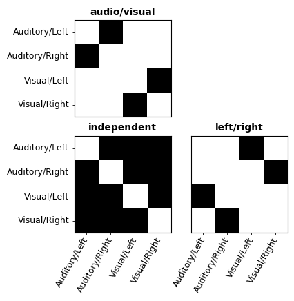
Model rdms¶

This is a simple example with basic model RDMs

[16]:

from rsatoolbox.rdm import get_categorical_rdm

[17]:

rdms_model_in = get_categorical_rdm(['%d' % x for x in range(4)])
rdms_model_lr = get_categorical_rdm(['l','r','l','r'])
rdms_model_av = get_categorical_rdm(['a','a','v','v'])

model_names = ['independent', 'left/right', 'audio/visual']

# append in one RDMs object

model_rdms = rdms_model_in
model_rdms.append(rdms_model_lr)
model_rdms.append(rdms_model_av)

model_rdms.rdm_descriptors['model_names'] = model_names
model_rdms.pattern_descriptors['cond_names'] = cond_names

[18]:

rsatoolbox.vis.show_rdm(model_rdms, rdm_descriptor='model_names', pattern_descriptor = 'cond_names')
None

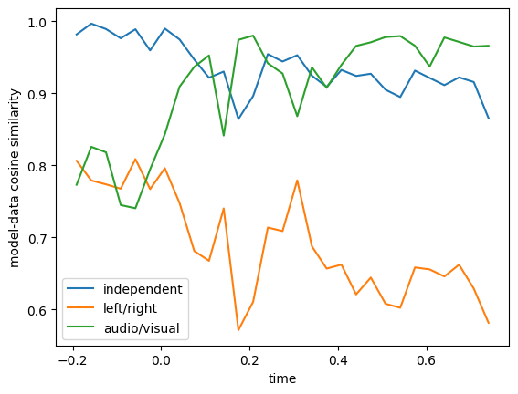
data - model similarity across time¶

[19]:

from rsatoolbox.rdm import compare

[20]:

r = []
for mod in model_rdms:
    r.append(compare(mod, rdms_data_binned, method='cosine'))

for i, r_ in enumerate(r):
    plt.plot(rdms_data_binned.rdm_descriptors['time'], r_.squeeze(), label=model_names[i])

plt.xlabel('time')
plt.ylabel('model-data cosine similarity')
plt.legend()

[20]:

<matplotlib.legend.Legend at 0x2c54fb820>

Temporal RSA¶

Load temporal data¶

The `rsatoolbox.data.TemporalDataset` class¶

convenience methods¶

`rsatoolbox.data.TemporalDataset.split_time(by)`¶

`rsatoolbox.data.TemporalDataset.subset_time(by, t_from, t_to)`¶

`rsatoolbox.data.TemporalDataset.bin_time(by, bins)`¶

`rsatoolbox.data.TemporalDataset.time_as_observations(by)`¶

create RDM movie¶

from here on¶

Model rdms¶

data - model similarity across time¶

rsatoolbox

Navigation

Related Topics

Temporal RSA¶

Load temporal data¶

The rsatoolbox.data.TemporalDataset class¶

convenience methods¶

rsatoolbox.data.TemporalDataset.split_time(by)¶

rsatoolbox.data.TemporalDataset.subset_time(by, t_from, t_to)¶

rsatoolbox.data.TemporalDataset.bin_time(by, bins)¶

rsatoolbox.data.TemporalDataset.time_as_observations(by)¶

create RDM movie¶

from here on¶

Model rdms¶

data - model similarity across time¶

The `rsatoolbox.data.TemporalDataset` class¶

`rsatoolbox.data.TemporalDataset.split_time(by)`¶

`rsatoolbox.data.TemporalDataset.subset_time(by, t_from, t_to)`¶

`rsatoolbox.data.TemporalDataset.bin_time(by, bins)`¶

`rsatoolbox.data.TemporalDataset.time_as_observations(by)`¶